ZZBrowse
ZZBrowse is an interactive R/Shiny web application for GWAS and QTL visualization. In this post, we describe our enhancements to the original ZBrowse developed by the Baxter Laboratory.
ZZBrowse is an interactive R/Shiny web application for GWAS and QTL visualization. In this post, we describe our enhancements to the original ZBrowse developed by the Baxter Laboratory. (For an overview of its basic functionality, please refer to the landing page.)
1. Comparative GWAS Visualization
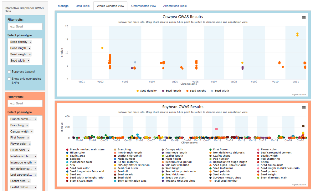
Each ZZBrowse view now supports simultaneous visualization of GWAS data for two species, with Species 1 (here, cowpea) framed in blue and Species 2 (soybean) in orange.
2. Macrosynteny blocks
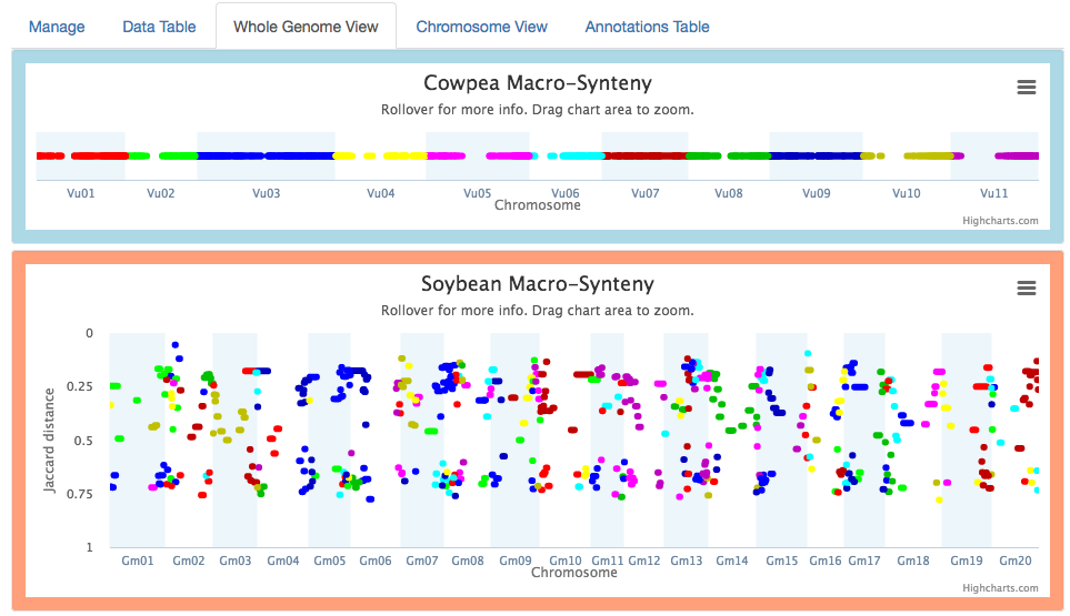
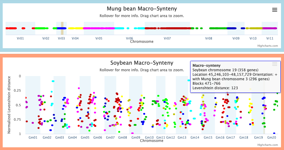
The Whole Genome and Chromosome views now plot macrosynteny blocks v. a syntenic distance metric (Levenshtein or Jaccard). The cowpea v. soybean example below reveals distance clusters corresponding to two whole genome duplication events, an earlier one around 0.70 and a more recent one around 0.25.
3. Linkouts and Genomic Linkages
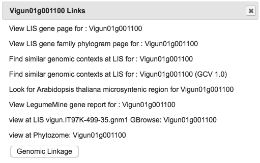
In the Chromosome view, clicking on a gene pops up a menu of linkouts. Click any of these to open its link in a new window.
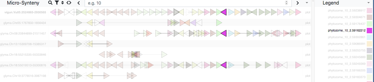
For Species 1, the menu also has a Genomic Linkage option. Clicking this calls the Genome Context Viewer to identify similar regions in Species 2 (defined by the number of matching and non-matching neighboring genes). Matching genes are color-coded by gene family in rainbow order (relative to their Species 1 sequence), illustrating the degree of synteny between the two species. If more than one similar region exists in Species 2, the Related Regions menu lets you choose which one to view.
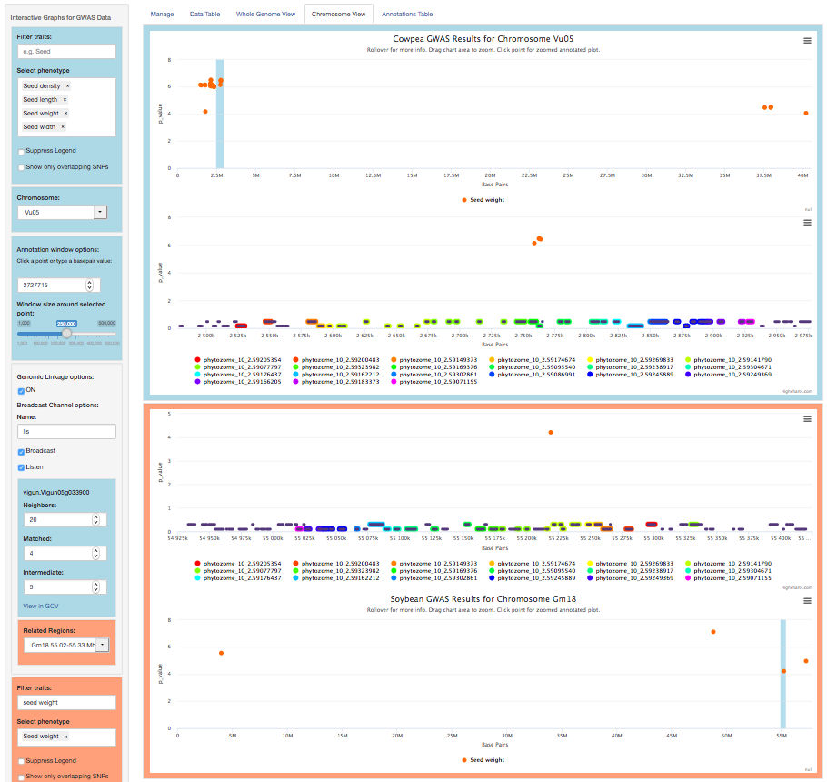
In the example above, there is considerable synteny between regions of cowpea chromosome 5 (2.5-2.9 Mbp) and soybean chromosome 18 (55.0-55.3 Mbp). The GWAS data (Manhattan plots) show significant associations for seed weight in both regions.
4. Using Macrosynteny to search for Genomic Linkages
The macrosynteny chart can serve as a guide for identifying likely related regions of the two genomes. To do so,
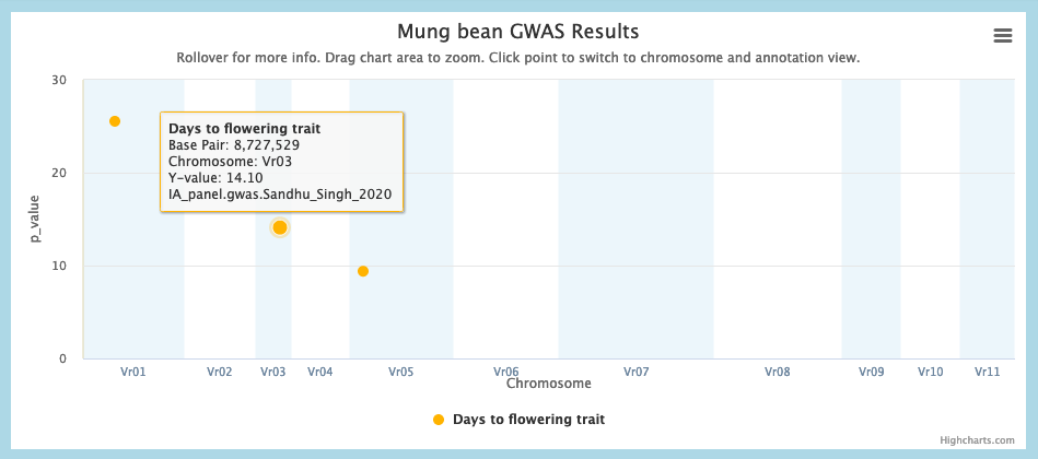
1. In the Whole Genome view, choose a GWAS peak for a trait of interest in Species 1, and call its location L1.
Example: Days to flower at 8.7 Mbp of Mung bean chromosome 3.
2. In the macrosynteny chart, identify regions of the Species 2 genome (L2) that are macrosyntenic to L1. There may be multiple L2 regions. You may filter on a given Species 1 chromosome to make the L1-L2 relationships more visible.
Example: the rightmost dark blue macrosynteny block of Soybean chromosome 19, from 45.2-48.1 Mbp, is macrosyntenic to blocks 471-766 of Mung bean chromosome 3, which overlaps our selection.
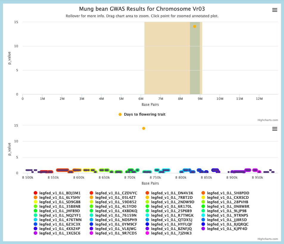
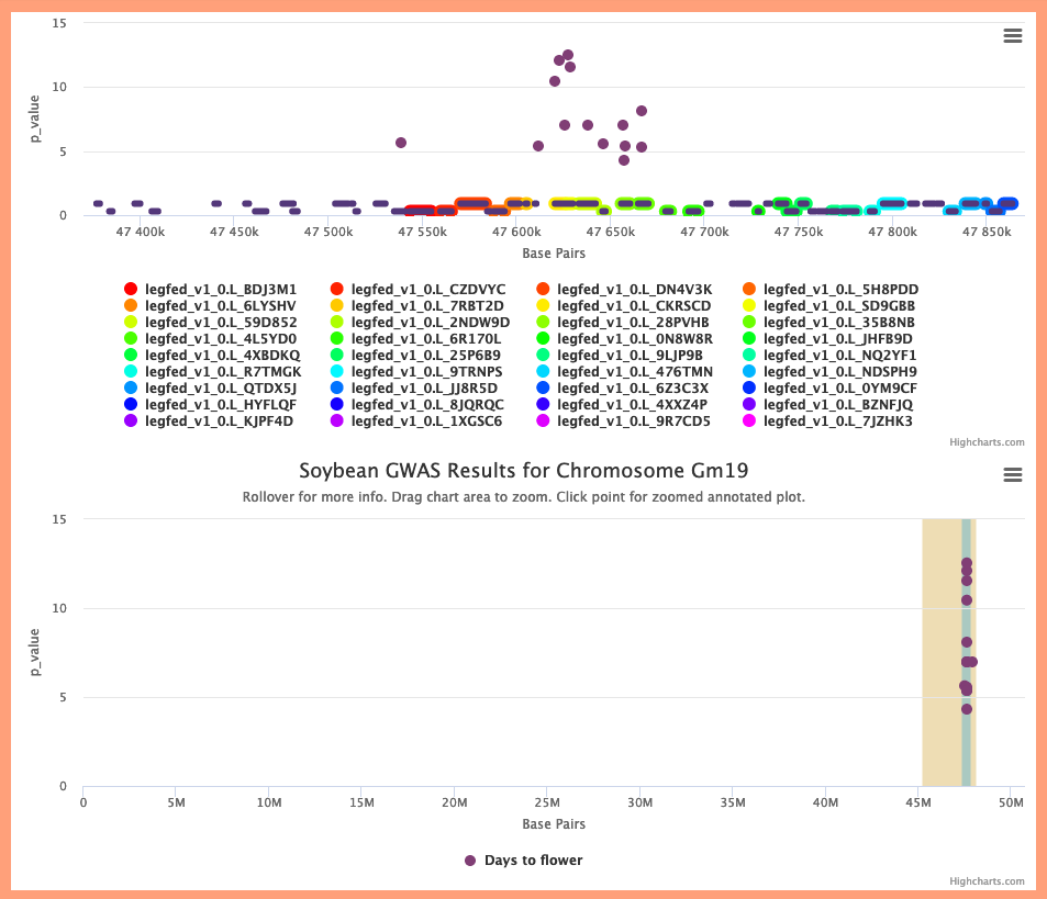
3. Again refer to the Whole Genome view. If any GWAS peaks for related traits exist in L2, click on the original GWAS peak in L1 to go to the Chromosome view. Then click on a gene in L1 to look for genomic linkages between L1 and L2.
Example: In the Chromosome view, click the Mung bean gene vigra.Vradi03g07280, then the Genomic Linkage button. Either of the (adjacent) related regions in Soybean chromosome 19 overlaps the Days to flower GWAS peak there.
5. Communication with the Genome Context Viewer
The Genomic Linkages feature also enables communication between ZZBrowse and the Genome Context Viewer (GCV). For example, when Broadcast is enabled, clicking a gene family legend item like  highlights genes belonging to that family in the GCV.
Similarly, when Listen is enabled, mousing over an item in the GCV highlights the corresponding item(s) in ZZBrowse.
The Show in GCV link tells the GCV to focus on the same region of the Species 1 genome displayed in ZZBrowse.
Other New Features
Importing local GWAS data: The original ZBrowse allowed loading your own local GWAS data files, but assigned each to a new, standalone dataset. Our implementation does not create new datasets on the fly, but instead adds user data to existing ones. We hope this feature will benefit researchers desiring to superimpose their own bleeding-edge GWAS data on previously published results.
We provide GWAS datasets for common bean, cowpea, mung bean, peanut, pigeonpea, and soybean, while the Medicago truncatula and Arabidopsis thaliana datasets are initially empty (a few traits are available through the Remote Trait Files selector).
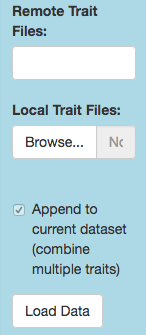
To add your own local GWAS data, first prepare them as a delimited text file with a header row listing the column names. Required columns are chromosome, position, trait (= phenotype), and p-value (or other significance metric) for each SNP, but you may include others. Click the Local Trait Files/Browse button to specify which file(s) to load, then click the Load Data button to append the GWAS data. Finally, tweak any details (such as whether to take the negative logarithm of the reported p-value) through the Manage tab.
Importing local QTL data: We provide QTL datasets for common bean, cowpea, and peanut. To add your own QTL data, prepare a similar delimited text file as for GWAS data, but including columns for start and end position of the QTL interval. In the position column, put the center position of the interval.
Application state: The URL automatically reflects the current state of ZZBrowse, allowing you to easily save a result and replicate it later. For example, if you want to share an interesting genomic linkage with a colleague, just copy the current URL and paste it into an e-mail message. They can then launch ZZBrowse and recreate the same view.
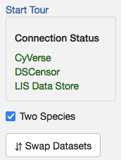
Tour: The Start Tour link (in the Manage tab) launches a guided tour (or tutorial) of ZZBrowse.
Connection Status: This panel (also in the Manage tab) indicates when remote data sources are unavailable, relieving user angst.
Two Species: Toggles display of Species 2, macrosynteny, and genomic linkages (for “original ZBrowse” mode).
Swap Datasets: Exchanges Species 1 and Species 2.